Note: This Document was converted to HTML with Microsoft Word. However, MS Word is not capable of producing readable HTML. So it required much manual editing to get at least this status which is not perfect indeed. I appologise for the figures that were heavily abused by MS Word. Copyright 2000 Christof Kaiser. All rights reserved. See my homepage for my email address. Download the whole thesis as on zip archive.

Table of Contents

Title Page	i
Table of Contents	ii
List of Figures and Tables	iv
Abstract	v
Acknowledgements	vi

1 Introduction *
2 Literature Review *

List of Figures and Tables
 

Figure 1: The greedy algorithm cannot find the optimal solution for this graph.	14
Figure 2: This graph with the indicated start configuration lets Teitz-Bart fail as well as GRIA.	16
Figure 3: Example for three primary extents	18
Figure 4: Leaving a Local Minimum with Simulated Annealing	20
Figure 5: Selection function.	26
Figure 6: Creating a new chromosome by crossover	27
Figure 7:Optimal Locations for 7 Additional Pharmacies in Western Australia. Population Dataset A	37
Figure 8: Optimal Locations for 5 Additional Pharmacies in Western Australia	39
Figure 9: Effects of additional pharmacies. (GRIA with population dataset B)	40
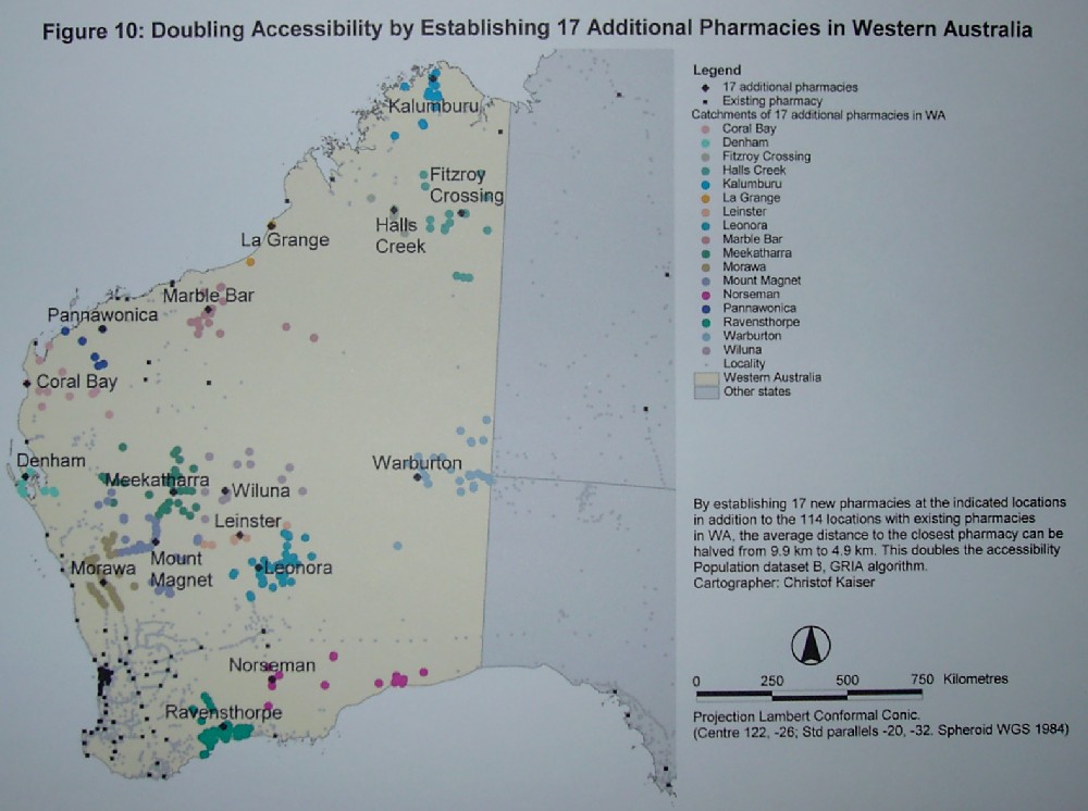
Figure 10: Doubling Accessibility by Establishing 17 Additional Pharmacies in Western Australia	41
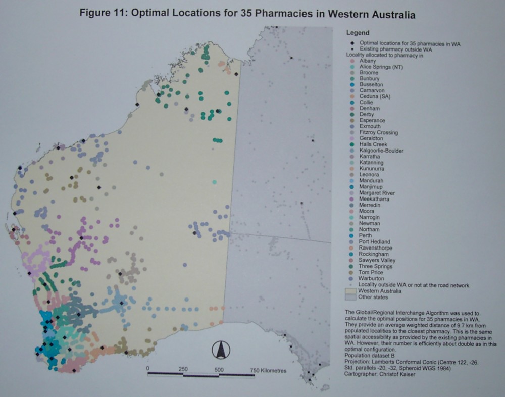
Figure 11: Optimal Locations for 35 Pharmacies in Western Australia	43
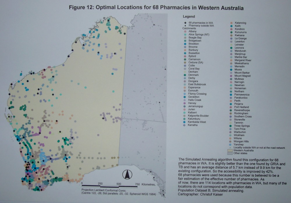
Figure 12: Optimal Locations for 68 Pharmacies in Western Australia	45
Figure 13: Average distances for optimal configurations of 1-70 pharmacies in WA. Calculated using GRIA and population dataset B.	46
Figure 14: Locating 35 pharmacies in WA. Results of different algorithms.	47
Figure 15: Results of different algorithms for locating 68 facilities.	48
Figure 16: Finding positions to establish additional facilities by using different algorithms. (Population data B)	49
Table 1: Runtimes for locating 50 facilities from scratch in WA	50

Abstract

Location theory deals with the search for spatially optimal positions for facilities. One of the standard problems of location theory is the p-median problem where a number of p facilities should be positioned to satisfy demand coming from point sources. The distribution of the p facilities is optimal, if the weighted distance from the points of demand to their closest facilities is minimised. This problem is computationally very hard. Different algorithms exist to find good solutions. In this study, six different algorithms are implemented: Greedy, Drop, Global/Regional Interchange Algorithm (GRIA), Teitz-Bart, a Genetic Algorithm and Simulated Annealing. Some of these are classic algorithms; others are new approaches to the p-median problem. The algorithms are compared in terms of quality of the solution and computation time. It is found that GRIA is usually a good choice both in terms of quality of the solution and the computation time. However, occasionally other algorithms such as Simulated Annealing find better solutions. Data captured for the Accessibility/Remoteness Index of Australia (ARIA) is used to optimise the positions of pharmacies in Western Australia. It is found that another distribution of these facilities would lead to a significantly smaller average distance to the closest pharmacy and so to a higher spatial accessibility. Moreover, establishing a small number of additional pharmacies could also lead to a large increase in accessibility without relocating existing pharmacies. The existing configuration of pharmacies in WA is far from optimal in terms of spatial accessibility for the population.

Acknowledgements

I whish to thank

• Brett Bryan for the supervision
• Danielle Taylor for help with the ARIA data.

The spatial locations of facilities determine if these are easy to reach from the points of demand. This holds for many applications such as warehouses, which should be reachable for their customers, mobile phone towers that must be in range of the handsets, recycling stations to collect rubbish from households, or the office location of an insurance agent who needs to visit clients.

The consequence of facilities at not optimal locations is low accessibility. That means that they are more difficult to reach from demand points. Insufficient accessibility can become a major problem in remote areas where the demand for a service by the population is too low to attract a facility but the travel efforts necessary to reach an alternative service are large. So especially for remote areas an optimal spatial distribution of facilities according to the distribution of demand and the travel efforts can produce a greater accessibility with the same number of service points.

Large parts of Australia are barely populated and experiences great disadvantages in the provision of facilities and services such as health, banking, and educational facilities. Therefore it is desirable to examine if a different spatial distribution of the facilities could increase the accessibilities of those, or where additional facilities should be put out to gain maximum benefits by reducing the remoteness of spatially disadvantaged localities.

To do so, several spatial location/allocation for the p-median problem are implemented and compared in this study and used to optimise the location of pharmacies in Western Australia.

2 Literature Review
Location theory is a well-established field of research. In the following, an overview of past research is given. Due to the scope of this study, the p-median problem and algorithms to solve it and services in rural Australia are looked at in particular.

2.1 Services in Rural Australia
The Accessibility/Remoteness Index of Australia (ARIA) provides a measurement of remoteness or accessibility for the whole of Australia (Commonwealth Department of Health and Aged Care 1999). It is based on the road distance from localities to service centres of different categories. One output is a continuous grid with values indicating the accessibility or remoteness at every point of the whole of Australia. For ARIA, the geographical positions and numbers of different kinds of services such as GPs, pharmacies and educational institutions were captured in a GIS database as well as point population data derived from different sources. Also all road distances from every known locality to every point hosting a service were calculated on a road network. These datasets are indispensable for the present study that tries to optimise the location of services.

2.2 Location Theory and Optimisation
The need to spatially locate facilities in an efficient way arises in many situations. A variety of academic disciplines are dealing with this problem. Operations Research looks at location theory to optimise business decisions; Geography has a broader look at the issue and Mathematics sees the problem as part of graph theory.

Location theory can be seen as one of the foundations of social geography.

Thünen (1826) developed a theory of different land uses based on the concept of transport costs. These costs that grow with the distance are the major factor for the selection of locations for different agricultural land uses.

A classical work by Christaller (1933) introduces an optimal pattern of central places that have central facilities. It then tries to identify this hexagon-pattern in the distribution of real world cities. Christaller develops the theory in a deductive way; he believes that the spatial structure in the real world must be based on the same principles and therefore leads to the same result. However, the theory widely assumes that the space is uniform and does not have areas that are more or less suitable for the development of cities due to natural conditions such as mountains or rivers.

Applications of Location Theory to find suitable if not optimal locations have a broad spectrum. They include locating benefit posts that distribute welfare and health benefits (Nascimento and Beasley 1993, p. 1063), locating warehouses (Kuehn and Hamburger 1963, p. 643), freight transport between different production facilities (Klincewicz 1990) and choosing positions for exchanges in a telecommunication network (Hakimi 1964).

Location theory recognises a number of problem types that are often similar but not identical.

2.3 P-Median Problem
The p-median problem is one of the basic questions of location theory and is as follows: The spatial distribution and the amount of demand for a certain service or facility is known. The task is to find locations for a given number of facilities that satisfy the demand. The facility locations are optimal, if the weighted travel efforts from the demand points to the nearest facilities are minimised. The problem is uncapacitated, which means that a facility can match any amount of demand necessary.

2.4 Related Problems
In addition to the pure p-median problem, also known as the uncapacitated warehouse location problem, a huge variety of similar problems exist. However, the algorithms to solve those can be quite different.

In the capacitated warehouse problem, each warehouse or facility can only satisfy a maximum amount of demand whereas in the p-median problem no such limit exists. Again, the total effort to get from the sources to the warehouses or facilities is to be minimised (Kuehn and Hamburger 1963).

The p-centre or minimax problem tries to minimise the maximum distance from the demand points to the facilities rather than the average distance. This may be desired for emergency services where the respond time for the place furthest away still must be reasonably short (Plesnik 1987). Several modifications of p-centre problem exist. Daskin and Owen (1999) introduced the problem to cover a given fraction of the demand with a maximum distance to the facility with a minimum number of facilities as well as covering a given fraction in such a way that the distance to the closest facility is minimised.

The p-median or minisum problem can be extended to account for regional constraints to the p-median problem (Church 1990). With this, every region must receive between a lower and upper limit of facilities. This accounts for political subdivisions. Chardaire and Lutton (1993) extended the p-median problem to account for different types of located facilities that interact such as telecommunication terminals that are connected to concentrators, which are connected to each other. Densham and Rushton (1996) worked on a p-median problem where every facility needs a minimum workload.

2.5 Benefits of Optimal Facility Locations
The result of the p-median problem are optimised facility locations that provide an optimal accessibility for the given number of facilities. From a customer’s point of view, the services are easier to reach than in any other configuration. From a service’s view, the spatial configuration of facilities is optimal to address customer’s demand. For this study, the term spatial accessibility means the reciprocal of distance to the closest facility. So if the distance is halved, the accessibility is doubled.

2.6 Problem Definition p-median
This section defines the p-median in a more mathematical way.

Candidates or candidate locations are places that are suitable to establish service facilities. Service facilities cannot be erected outside candidate locations. A configuration is a set of usually p candidates that are proposed to get a service facility. However, during the optimisation process the configuration might consist of a different number. Every configuration that has exactly p facilities is a solution for the p-median problem. The optimal solution is a configuration that has the minimal cost. Every p-median problem has at least one optimal solution but there can be more if more than one configuration with the minimal cost exists.

The input data for an algorithm to solve a p-median problem are

• A finite number of demand points with demand values specifies the location and amount of demand that needs to be satisfied.
• A finite number of candidate locations. These are the only positions where facilities can be established.
• Distances between demand points and candidate locations. Depending on the problem, they can be calculated from a network or Euclidian distances. The distances are measures of impedance, so they can be time distances or monetary costs as well as kilometres.

The Objective Function is the essential part of every optimisation. This function evaluates the quality of a solution and returns a number value for it. An optimisation algorithm tries to find a solution for that the objective function returns a minimal (or maximal) value.

For this study, the objective function is the total cost from every point of demand to the closest facility of the configuration. The cost is weighted or multiplied by the demand of the point.

A constraint is that each demand must be assigned to its closest facility. The total number of facilities is p.

The result of the optimisation process is a configuration with p facilities and the total cost calculated by the objective function for this configuration. For ease of understanding, it might be helpful to calculate the cost per demand.

2.6.1 Mathematical Definition
Narula, Ogbu, and Samuelsson (1977) formulated the p-median problem as follows:

is the value of the objective function. This is to be minimised.

is the number of locations of service recipients or demand locations

is the number of facilities to be located

is the amount of demand at location i

is the distance or cost from demand location i to facility location j

is the decision or spatial allocation variable. It is 1 if the demand at location i is allocated to a facility located at j, 0 otherwise.

is the demand at point i;  is the shortest distance from demand i to candidate location j; if the demand from point i is satisfied by a facility at candidate location j. The set of the demand points is the same as the candidate points, therefore both i and j have the same range from 1 to n. If a location has a facility, this is the closest to the demand from the same point as the distance is nil. Therefore the number of facilities p can be counted by calculating .

2.6.2 Extensions
The definition of the problem can be extended in a natural way to account for facilities that are static or fixed. That means they must be considered if the shortest distance is calculated, but they are not part of the optimisation process.

Unlike in the definition by Narula, Ogbu, and Samuelsson (1977), the number of candidate locations and demand points can be different.

The total demand is constant throughout the optimisation process. Hence minimising the total cost is equivalent to minimising the average cost per demand unit. The average cost per demand unit might be a more intuitive result as it corresponds to the real world. For example, it can be the average kilometre distance that must be travelled to reach the closest facility.

2.7 Complexity of the p-Median Problem
The complexity of algorithms is measured in the O() or ‘Order of’ notation that states the principle computation time as a function of the input data size n. O(1) is constant time, that is, the computation time does not vary with the size of the input data. If the runtime is O(n) it grows proportional with the input data. In the case of O(n²), the computation time increases by a factor of four if the problem size is doubled.

In computer science, algorithms are divided into two classes according to their complexity. Algorithms with an order that can be expressed as a polynomial such as O(n^k) (with constant k) are called P-hard. This group includes algorithms with computation times of O(1), O(n log n) for sorting using the quick sort algorithm or O(n¹⁵).

The other class contains algorithms which computation time exceeds any polynomial boundary. It is called NP-hard (non polynomial). Typical orders of these very time consuming algorithms are O(kⁿ) with k constant and greater that 1. This is also referred to as ‘exponential time’. An O(2ⁿ) algorithm needs twice as much computation time to terminate if the problem size is only increased by one. Hence it is impossible to solve big problems even with enormous computer power.

Until now it is not proven, that it is impossible to deduct NP-hard problems to P-hard ones (Pelletier 1998). Doing this would make them much easier to handle. However, it appears to be a well-established fact in theoretical computer science that P-hard and NP-hard problems are not related.

For many combinatorial problems such as the well-known Travelling Salesman Problem only NP-hard algorithms are known.

Kariv and Hakimi (1979, p. 540) showed that the ‘general p-median problem is NP-hard’. As mentioned above, it is not yet proven that the problem classes NP and P are different. Therefore Kariv and Hakimi state ‘that there exists an O(f(n,p)) algorithm for finding a p-median of a general network where f(n,p) is a polynomial function in each of the variables n and p only if P=NP’.

2.8 Principle Approaches and their Characteristics
Algorithms solving p-median problem can be divided into three principle groups: Algorithms that guarantee to find the optimal solution, here called optimal algorithms, algorithms that are based on heuristics and find a good but not always optimal solution without trying all possibilities and algorithms that use a certain amount of chance to find a good solution.

2.8.1 Optimal Algorithms
To find an optimal solution of a p-median problem is NP-hard as mentioned above. Therefore all algorithms that find the optimal solution will need a huge amount of computing time if the problem gets bigger. However, optimal algorithms may be used for small problems and to benchmark other algorithms.

Combinatorial algorithms enumerate all valid possibilities of the given facility location problem and hence can find the optimal solution. Enumeration is a naïve approach for all combinatorial problems. For the p-median problem, enumeration was suggested as early as 1964 by Hakimi when the problem was firstly mentioned. Due to its obvious outranges computation time as an NP-hard algorithm he already discarded it as an impracticable way of solving the problem. However, for very small datasets the algorithm can be very helpful because it guarantees that the optimal solution is found and it is easy to understand and implement. The number of different configurations isif n is the number of candidate locations and p is the number of facility locations to be selected.

Given the case, that two facilities are to be chosen out of four facility candidates named A, B, C, D, the complete enumeration contains  configurations:

A, B
A, C
A, D
B, C
B, D
C, D

A mathematically more sophisticated optimal algorithm uses Lagrangian relaxation, applied to the p-median problem firstly by Narula, Ogbu, and Samuelsson 1977. This technique ‘relaxes’ one of the constraints of the p-median problem. Usually the constraint that a candidate is part of a configuration (1) or not (0) and a candidate’s membership to one configuration is a float value rather than either 0 or 1. By doing this, optimisation techniques for continual problems can be applied to the modified problem. However, the problem remains NP-hard and therefore Lagrangian relaxation is not suited for greater problems even with the power of recent computers. Church and Sorensen (1996, p. 173) note that this may be the reason why this technique is not included as a Location/Allocation function in Esri’s ArcInfo.

2.8.2 Heuristic Algorithms
Heuristic algorithms for combinatorial optimisation use rules of thumb to find good if not optimal solutions. They cannot guarantee to find the optimum but they usually find a good solution. Heuristic Algorithms do not try every solution as the enumerative approach. Several heuristics exist that are more or less successful in approaching the p-median problem. Good heuristic algorithms usually produce good solutions; however they can yield poor results in special cases. This is problematic because nothing is known about the quality of the solution. Poor solutions can only be identified by using different algorithms for the same problem.

For the p-median problem, many heuristics are known and some of them have several sub-species.

2.8.2.1 Greedy/Myopic/Add
The Greedy Algorithm, also referred to as Myopic or Add Algorithm, was first suggested by Kuehn and Hamburger (1963, p. 645) for a slightly different problem as well as in 1966 by Feldman, Lehrer, and Ray.

It follows a very simple strategy: within each iteration it puts a new facility at the location whichever reduces the total cost most. It starts with an empty configuration and stops if the configuration reaches the desired number of p facilities. Once a facility is established in the configuration, it is never moved. The algorithm always terminates and the computation time is known and small. However, the Greedy Algorithm is very likely to get caught in a local optimum. Consider the linear network of five nodes in figure 1 with a demand of one for each point and a distance of one between every two neighbour points.

All points are facility candidates. The first point the Greedy algorithm chooses is C because it has the minimal cost of a one-point configuration of 6. The second point can be any of A,B,D,E since a new service at any of these points results in a total cost of 4. However, the global optimum of a two-point configuration is B and D and has a cost of only 3. The Greedy algorithm is simple, but can easily be caught in a local optimum. However, it is rather fast and the time needed is determined only by the size of the input data such as number of candidate locations and demand points. So every problem of the same size needs the same time, the algorithm does not need longer if problem described by the data is difficult.

The Greedy strategy might be observed in reality if independent entrepreneurs establish their services of the same kind independently. Everyone will establish the new business (such as a Deli) at a place that is most accessible for the customers considering the existing competitors. But the resulting configuration will often be suboptimal in terms of overall accessibility.

2.8.2.2 Drop
The Drop algorithm is based on the naïve drop heuristic mentioned by Chardaire and Lutton (1993, p.186). Initially, all candidates are part of the configuration. In each iteration one candidate is removed until only the given number of p candidates is left in the configuration. In each iteration the candidate that is dropped is the one that produces the smallest possible cost increase of all candidates in the configuration if removed.

This strategy is the reciprocal of the Greedy/Myopic approach that adds one candidate to the configuration in each iteration step. Like the Greedy algorithm, it is fast, simple and tempted to return a sub-optimal result.

The Drop strategy might appear in reality if a company reduces its number of branches by always shutting down the one, which affects the overall accessibility least at that stage.

The Maranzana or alternating algorithm is known since 1964 (Maranzana) and is superior to the add and drop approaches.

2.8.2.3 Teitz-Bart
Teitz and Bart developed a successful algorithm for solving the p-median problem as early as 1968 which is also known as the Bump-and-Shift algorithm. It is, together with GRIA, one of the standard algorithms for this problem. It starts with an arbitrary configuration of p candidates. All unused candidate locations are kept in a pool. The idea is to exchange one location of the configuration with one of the pool if this leads to a smaller cost. If more then one candidates of the pool does so, the one that results in the smallest total cost is used. So every location of the configuration is swapped successively with every location of the pool and the change is accepted if the cost decreases. The algorithm terminates, if there is no pair of a pool and a configuration location left that would decrease the cost if swapped.

This algorithm is heuristic; it can be trapped in local optima. A constructed graph for this shown in figure 2. The distance between two neighbour nodes is always 1; the demand is 2 at node A and 1 at all other nodes.

If the 2-median problem is to be solved and the starting configuration is B and E, Teitz-Bart does not find the optimal solution A, D. However, for real-world problems Teitz-Bart appears to be very successful in finding the optimal solution as found by Narula, Ogbu, and Samuelsson (1977, p. 711).

It is much more likely to find the optimal solution than the Greedy or Drop algorithm. The runtime cannot be predetermined because the number of swaps needed varies. Some problems will incur a small number of efficient swaps. Other problems of the same size may need more swaps because the increase in accessibility per swap is smaller.

2.8.2.4 Global/Regional Interchange Algorithm
It was not until 24 years later that Densham and Rushton (1992a) came up with a new heuristic algorithm that is a few times faster than the Teitz-Bart one and also produces good quality results. This Global/Regional Interchange Algorithm (GRIA) combines two different heuristics but is still based on classical heuristic optimisation. It combines two old heuristic strategies of the Teitz-Bart algorithm from 1968 and one developed by Maranzana in 1964. GRIA applies both heuristics consecutively in each iteration. It starts with an arbitrary configuration of p candidates. During the global interchange, the facility of the configuration which’s removal increases the total cost least is removed. It is substituted by the candidate that produces the greatest cost decrease if added. The change is only accepted if the overall cost is decreased by the substitution. The global interchange is somewhat similar to the Teitz-Bart algorithm.

The other step in the iteration is the regional interchange. For every candidate in the configuration, its primary extent is calculated. The primary extend are all those candidate points that would be allocated to the very facility if they were demand points as shown in figure 3. For every primary extend, all members are tried as facility to see which one creates the smallest overall cost. This is then used instead the former candidate. The regional interchange is similar to the Maranzana algorithm.

The global and then the regional interchange are performed on each iteration. The algorithm terminates, after an iteration did not result in a change during the global nor the regional interchange.

The graph in figure 2 with the given start configuration lets GRIA fail as Teitz-Bart before. No global interchange is performed as well as any regional interchange within the primary extents of the candidates of the arbitrary configuration. Hence the algorithm stops with a total cost of 5 without finding the optimal solution with a cost of 4.

The quality of the solutions and the likelihood of local optima are similar to those of the Teitz-Bart approach (Densham and Rushton 1992a). The advantage of GRIA is that is usually several times faster.

Densham and Rushton (1992b, p. 302) claim that the computation time of GRIA approximately only increases linearly with the problem size. A complexity of only O(n) is a very good for solving the p-median problem.

2.8.3 Randomised Algorithms and Artificial Intelligence
The optimal and heuristic algorithms mentioned above are deterministic. The same input data always leads to the same result and computation time. A different class of algorithms uses a certain amount of chance as part of their strategy. Sometimes during the optimisation changes occur that increase the cost contrary to the optimisation goal. By doing this, the algorithm can jump out of a local optimum. However, this makes the search less straightforward and hence more time consuming.

2.8.3.1 Genetic Algorithm
Genetic algorithms (GAs) emulate a natural evolution process to find good solutions and can be used for most optimisation problems. They start with a number or population of arbitrary solutions. This population is then substituted by a new generation of solutions that usually have a better quality. To do so, the quality or fitness of every solution or individual is calculated. The next generation is generated by recombining, mutating and copying those individuals that have a good fitness. However, this selection process as well as the mutation and crossover methods are randomised. The process of substituting the former generation by it’s offspring that has a better fitness is continued until some termination criterion is met such as no further notable increase in fitness or a maximum number of generations is reached. Genetic algorithms have proven to be a good choice of optimisation problems if no successful problem specific strategy is known (Goldberg 1989).

2.8.3.2 Simulated Annealing
Simulated Annealing is an optimisation technique that is linked to the process of crystallisation of melted metals during the cooling process. It was mentioned as early as 1953 by Metropolis et al. A certain amount of random changes are introduced to an established heuristic algorithm to reduce the risk of getting trapped in a local optimum. An existing heuristic algorithm that only accepts changes if they decrease the total cost such as Teitz-Bart can be modified to a simulated annealing approach. A temperature is introduced that decreases over time according to a given non-linear function or table. A change of the configuration that decreases the total cost is always accepted like in the heuristic algorithm. But also if the modification increases the cost, it is performed by a probability determined by the temperature and the cost increase. Chances of a cost increasing change to be accepted are highest for high temperatures and small cost increases. So in the beginning, when the system is still hot, changes that increase the cost are accepted relatively easily. Latter on, the probability of these changes, that contradict the optimisation objective of minimisation, to be performed, decrease. French (1994) states equation 1 as the standard to calculate the probability of accepting a certain change where p is the probability, ?c is the change in cost and T is the current temperature.

A heuristic that only allows modifications that decrease the cost function cannot leave a local minimum as shown in figure 4. The algorithm is trapped at solution 1 which is obviously a local minimum. But by chance, the simulated annealing algorithm can accept the cost increasing change to solution 2. From there, the global minimum 3 can be reached using the standard downhill strategy

2.9 Algorithms in Current GIS Software
With the p-median problem being a classical Operations Research task with geographical relevance, it can be expected to be solved by standard GIS packages. However, this is not the case. This might be due to the huge variety of location/allocation problems. To offer an algorithm for the p-median problem is not always sufficient because many real world problems have several other constraints. So the likelihood that the p-median-solver exactly fulfils the requirements is small. And so the pressure to implement it is smaller.

2.9.1 Esri’s ArcInfo
The GIS ArcInfo includes a function to optimise the location of facilities that was firstly included in Version 7 of ArcInfo, which was released in 1996. The function remains unchanged in the current Version 8.

The command is called locateallocate and is part if the ArcPlot module. The main input data are points of demand, candidate points for facilities and a network that is used to travel between demand and facility points. The command offers the choice between the GRIA and Teitz-Bart algorithm. Since both algorithms require the distances between each pair of origin (or demand) and destination (or facility) points as input data, this all-shortest-path matrix must be generated by ArcInfo from the given network. Several algorithms exists to calculate a shortest-path matrix out of a network graph such as the well known All-Pairs Shortest Pairs Algorithm by Floyd-Warshall as cited by Ahuja, Magnati, and Orbin (1993, p. 146f). This algorithm has a runtime of O(n³). Esri does not document which algorithm is used to create the all-shortest-path matrix by the locateallocate command. However, it was experienced that the implementation needs huge amounts of temporary disc space during the calculations and tends to fail without any reason if the network becomes larger. Therefore the GRIA or Teitz-Bart algorithm itself is not started. It was experienced that the calculation of the all-shortest-path matrix already failed for a moderate street network of 4932 edges with 3598 demand points and 13 candidates. For this test, five locations out of the 13 candidates were to be selected.

2.9.2 Other GIS
Locality optimisation functionality is not included in ArcView 3.2 as well as in any of the extensions for ArcView offered by Esri including network analyst.

MapInfo up to Version 6 offers no algorithm to solve the p-median problem.

3 Methodology
This study has two objectives: to compare the performance of different algorithms for the p-median problem and to optimise the location of pharmacies in Western Australia in terms of accessibility. Therefore, the different algorithms described above as well as two newly developed ones were implemented and used with data of Western Australia.

3.1 Framework pmedian
The different algorithms described above were implemented in one Java (JDK 1.1) stand-alone application called ‘pmedian’ that is started from the command line. The specific parameters are in a separate manual of the program (Appendix A).

The traditional command line design was chosen to make it easy to use the tool in a scripting environment such as PERL. The computation time to solve larger p-median problems does not allow a fluent interactive user interface. A command line tool can easily be executed on a remote machine using telnet without stalling the user interface of the local machine.

A simple framework was implemented to read the input data from files. It can read the CSV (Comma Separated Values) format that is used for the ARIA input data. This text-based format is easy to import and export with many other programs such as spreadsheets and GIS.

All algorithms were extended to account for fixed service facilities, which are not to be changed and not part of the optimisation process. However, the algorithms have to account for the fact that they exist and satisfy demand. The concept of fixed facilities is essential for two reasons. Firstly, if a number of facility locations is to be optimised within a defined area such as a state, other (fixed) facilities might exist outside the area. A facility just outside the state is satisfying demand from within the state. This must be considered if the facility locations within the state are optimised. Secondly, if additional facilities within an area that already has some service locations are to be established, the existing ones must be taken into account when the new positions are optimised. Technically, the fixed facilities are only considered in the objective function. Hence they do not change the optimisation algorithm itself.
In addition to the traditional algorithms two new ones were developed based on the concepts of genetic algorithms and simulated annealing as described below.

3.1.1 Genetic Algorithm
Although the concept of GAs is easy to follow, it takes much effort to find problem specific adjustments of the algorithm such as the encoding of the solutions and details of the crossover and mutation process and suitable parameters. The details of the GA described here were developed by the author to make it suitable to solve p-median problems.

3.1.1.1 Chromosome Encoding
The standard way of encoding an individual or solution is as a bit string. This binary array is than decoded to get a solution. Applied to the p-median problem, a straightforward binary encoding would be to have one bit for every candidate and setting it to 1 if the candidate is a facility in the configuration. During the mutation and crossover process, the number of 1 in the bit array or the number of facilities in the configuration varies.

However, a valid solution of the p-median problem has exactly p facilities. Therefore most of the chromosomes that are created will not be valid solutions and only slow down the selection process.

Contrary to textbook solutions as described by Goldberg (1989, pp. 80) a non-binary encoding was used for the p-median problem since it is a combinatorial optimisation problem. A chromosome holds exactly p numbers. Each number specifies one candidate that is a facility in the configuration. So each configuration that is stored in a chromosome has exactly p facilities, although some facilities might be in multiple copies in the chromosome. To make the encoding of a configuration unique, the numbers are stored in a sorted way in an array. Otherwise the same configuration could lead to different chromosomes. This is unwanted to ensure an efficient crossover.

3.1.1.2 Fitness Function and Selection
The fitness of a configuration is calculated by the same cost function that is used for all implemented algorithms and described above. A low cost means a high fitness or quality of the solution (configuration) hence a high accessibility.

Within a genetic algorithm, the probability of selecting individuals as a basis for the next generation is usually determined directly by the fitness values. But for the p-median problem, the fitness or cost values of different solutions are often close together so that the probability of selecting a specific individual would only have slight differences. Therefore, the individuals are ordered by fitness and the probability is derived from the rank of the individual in its population. So the relation of the chance of the best individual to be chosen and the one of the individual at place 10 is always the same, regardless the absolute difference in fitness. Whenever an individual needs to be selected, a random variable x in the range of 0 and 1 is generated and a position in the sorted array is calculated according to equation 2.

Using this equation to select from an array of 100 objects, numbered from 0 to 99, leads to the probability distribution graphed in figure 5.

3.1.1.3 Crossover
The crossover produces one new child individuum from two parent solutions. The chromosomes can be combined by different methods ways to form a new one. Four different methods were implemented in pmedian. However, a standard textbook method proved to be successful. A cut-off point is chosen randomly between 0 and the length of the chromosome -1. The child chromosome is constructed by copying the information of the first parent from the beginning of the chromosome up to the cut-off point. The rest is copied from the second parent’s chromosome. After sorting the genetic information of the child, it can occur that some locations are recorded in multiple instances on the child chromosome. During the evolution process in the GA, these will disappear because they are normally not as fit as individuals without multiple copies of the same facility location. An example of this crossover principle with a cut-off at position 3 is shown in figure 6.

3.1.1.5 Promote Best
The very best individuals of a generation are copied to the next one without any changes. This ensures that the quality of the fittest individuum is never decreasing over the generations. Significant negative effects on the diversity of the offspring are unlikely as the percentage of the offspring that is produced by this method is often as low as 2%.

3.1.1.6 Parameters
Combinatorial optimisation with Genetic Algorithms is always a trade-off between a reasonable computation time and the risk to get caught in local optima. To find a solution in a rather straight way, the influence of random events must be small. A high mutation rate would also affect good solutions and, in most cases, worsen their quality. On the other hand, if not enough randomisation is used, the algorithm might get caught in a local optimum because the random changes are not big enough to find a rather different solution (see figure 4). Depending on the size of the population, less randomisation also leads to inbreeding because crossing similar individuals without sufficient random changes lets the whole population converge to similar individuals. The default parameters used for this study are: population size 200, termination after 200 generations without improvement of the best individual, the next generation consists of the best 2% of individuals of the last generation, 60% gained by crossover and 38% by mutating individuals selected from the last generation as described above. In the mutation, the probability for every information (i.e. facility location) to be changed is 20%. The crossover method is No. 4 which is the one described in this paper.

3.1.2 Simulated Annealing
Simulated Annealing algorithms are usually based on a heuristic. For this implementation, a heuristic based on Teitz-Bart was utilised. The genuine Teitz-Bart algorithm swaps a used candidate with a currently unused candidate that decreases the cost most. For this implementation of a simulated annealing, this was changed to the first candidate that reduces the cost. This was done to also find swaps that increase the cost and though can be accepted by chance in the annealing process. The temperature decrease was realised by multiplying the temperature with a cooling factor less than 1 in each iteration. The default initial temperature for this study is 500000 and the cooling rate 0.999.

The Teitz-Bart and GRIA algorithms without simulated annealing barely get trapped in local optima. Contrary, the arbitrary changes lengthen the time needed by those algorithms to find the solution. And for the unlikely event of GRIA or Teitz-Bart entering a local minimum, simulated annealing only jumps out by some chance. So the risk of destructing good solutions by simulated annealing or to lengthen the process is high compared to the benefits of the chance of leaving a local optimum because local optima are more a theoretical than practical problem for GRIA and Teitz-Bart. However, it happened that Simulated Annealing outperformed Teitz-Bart and GRIA as discussed in the results section.

Nevertheless, for questions similar to the p-median problem that have more constrains, simulated annealing can be very fruitful as experienced by Chardaire and Lutton (1993, p. 194).

3.2 ARIA Data
The optimisation of service locations is very sensitive to the input data. Great care must be taken when choosing these datasets. If no reliable or complete data is available, it might be a good idea to run the optimisation with slightly different datasets of the same area to see how these differences affect the result.

For this study, data from Western Australia was used. WA is a promising area for the optimisation of service locations because huge parts of the state are unpopulated. People living in these remote areas experience a very low accessibility to service locations. Since the travel distances to the next facility can be very large, an optimised configuration of service points might lead to a significant increase in accessibility.

3.2.1 Population Data
The p-median problem is based on spatially distributed demand values. For many applications, the total population is used as demand. Although this is reasonable in general, the demand can be specified more accurately in some special cases if the examined services are more demanded by certain parts of the population. This can be reasonable if the locations of aged-care facilities or female GPs are to be optimised.

For ARIA, population data of localities with a population of 200 or more from the 1996 census conducted by the Australian Bureau of Statistics (ABS) (1997) was assigned to localities provided by AUSLIG (2000). Population for smaller places is not available from the ABS. The AUSLIG data includes the positions and names that are ‘named on the 1:250,000 scale source material’ (AUSLIG 2000). It also includes named locations that are unpopulated such as road junctions. There are 1575 points in WA. Out of these, 168 have a population of at least 200 people for which the exact number is known from the ABS data and sums up to 1,538,239. The total population of WA according to the 1996 census (Australian Bureau of Statistics 1997) is 1,726,095. The population of every census district is known, but not those of the single settlements and towns. However, this population data of small towns is essential if the accessibility of services should be improved. Because the people in these places are unlikely to have a service nearby, they must travel several kilometres to the next facility and therefore have a significant impact on the over-all travel cost. Information about the distribution of the rural population is indispensable to reduce spatial accessibility disadvantages of these people by optimising the locations of services.

Different approaches were tried to estimate the population in places with fewer than 200 people. It is strongly suggested that these estimations are reviewed if the population data for smaller towns and communities cannot be acquired before the results are used.

It is believed that the use of the genuine ARIA population data is biased towards a better accessibility. This is, because the population dispersed into locations with under 200 people is not taken into account. But services are more likely to be found in larger towns. So parts of the disadvantaged population that do not have a facility in their own locality and therefore have to travel a notable distance are left out in this calculation.

Current and Schilling (1987) examined the effects of aggregated demand data on the solution of a p-median problem and found that the aggregation decreases the quality of the solution. Fotheringham, Densham and Curtis (1995) also found that aggregated demand data can corrupt the results of location-allocating modelling. The well known but unenviable modifiable area unit problem (MAUP), which occurs when data is spatially aggregated into arbitrary units such as administrative boundaries, also affects the solution of the p-median problem. In opposition to this, Murray and Gottsegen (1997) found that the quality of the solutions of p-median problems is stable when aggregated data is used. The chosen candidates can be different, if aggregated data is used, but the quality of the solution, which is the total cost, is very stable for both the aggregated and more detailed demand data.

For this study, the demand data was not further aggregated to reduce the computational complexity of the problem. However, it must be seen that the data as it is used is already aggregated to some extent since the population of urban centres is assigned to one point. But this population data issue is beyond the scope of this study.

3.2.1.1 Population Dataset A
The locations with a population of 200 and over from ARIA were combined with 41 points of smaller populations. The latter population numbers could be acquired from the 1996 Census data because remote communities are often treated as one Census District (CD). A comparison of the positions of these CDs and populated points with unknown population allowed mapping the known population of a CD to a point in most of the cases. By doing this, a total of 208 demand points with known population in WA was obtained. These have a total population of 1,545,003 people. Although 181,092 people of WA are left out in these numbers, this dataset has the advantage that only known population figures are used. Therefore no additional errors are introduced by estimating population for certain points.

3.2.1.2 Population Dataset B
Based on Population Dataset A, a more complete estimation of the distribution of the population was developed. Firstly, the population of non-urban CDs that only contained localities without known population was divided by the number of localities and assigned to them. Secondly, the population of 192 non-urban CDs that did not contain any locality point were added to the locality whichever was closest to the CD. The sum of the population attached to localities is 1,710,144 in 1285 localities, which is 15,951 less than the population of all CDs. The difference is believed to be due to mismatches of locality points and CD boundaries. If a locality with known population falls into wrong CD due a lack of spatial accuracy, the population of this CD is not assigned to any point since it is believed to be already included in the locality. However, the pmedian program ignores another 267 persons because these are assigned to 7 localities that are not connected to the road network and hence are not part of the distance matrix. Although the population total differs less than 1% from the sum calculated from the CDs, there are some uncertainties about the distribution. This is because some rural CDs have a huge area so that the population distribution within the CD will have an impact. Some localities are very close to the border of CDs so that they might fall in the wrong CD due to accuracy issues.

3.2.2 Service Points
The service point data will normally be more complete than the population data. This is, because the number of facilities is smaller than the number of population points and the information is binary instead of numeric. That means, a point has either a facility or not. The number of facilities at one point is not important because for this study the uncapacitated p-median problem is used. Therefore, a facility can satisfy every demand.

The result of the optimisation process is very sensitive to errors in the service point location data in remote areas. If a remote point with demand is regarded as a service point by mistake, the travel cost will be underestimated. If the point is regarded to be without a service facility by error, the total cost is overestimated. The impact of errors of remote points is more significant that those in urban areas, because the travel distance to the next facility is usually much greater.

3.2.3 Candidate Locations
Candidate locations are points that are suitable to establish a facility. Usually, these locations will be different from the already existing service points. However, if some candidate locations are already a service location, it is unlikely that the optimising algorithm would put out another facility at this point because it would not increase the accessibility.

If an existing configuration should be compared with an optimised configuration of the same number of facilities, all locations of the existing configuration should be included in the set of candidate locations. This ensures, that the existing configuration can be the output of the optimisation if it already was optimal. Hence for this study candidate locations are all localities in WA with a population of 200 or more as well as all locations of existing pharmacies. This is a total of 214 candidates.

3.2.4 Distance Matrix
All location/allocation algorithms need information about the distance or travel cost between the demand locations and the service or candidate locations. For this study an existing distance matrix of ARIA was used which was calculated using the road network. Hence the distance values are the shortest road distances between origin and destination point. It is essential that the demand points have a connection to a facility point because otherwise the travel cost cannot be calculated and hence must be set to infinite. Special care must be taken for islands, which naturally do not have a connection to the main road network. Incomplete or broken road networks are likely to produce artefacts such as unconnected demand locations or artificial detours. The distance matrix of WA from ARIA was corrected for two populated localities on islands. The sea distance to the closest point connected to the road network was weighted according to the ARIA standards (Commonwealth Department of Health and Aged Care 1999, p. 15). Distances within the same locality are ignored.

Note that the kilometre distance is only one possibility of assessing the impedance to travel between points. It also appears to be sensible to weight the geographical distance by the road condition in form of the average travel speed. So the travel cost could be expressed as a time value. Doing this, a 100 km journey on a sealed highway may raise the same cost as a 30 km journey on an unsealed track.

The used distance matrix of Western Australia has a file size of 55 MB if stored as text.

4 Results

4.1 Effects of Optimised Facility Locations on the Accessibility of Services in Western Australia
The described data was used with the algorithms implemented to optimise the locations of pharmacies in Western Australia. Unless mentioned otherwise, the GRIA was used to find good configurations.

4.1.1 Population Dataset A
The population dataset A was used as demand data to find good, if not optimal locations to establish new pharmacies in addition to the locations that already have at least one pharmacy in WA. These 114 locations with pharmacies as well as existing pharmacies in the neighbouring NT and SA lead to an average distance of 5.7 km for a person to travel to the closest service. This distance can be decreased rapidly by putting out only a small number of new pharmacies in the right locations. If only 7 extra locations get a pharmacy in addition to the 114 locations that already host one, the average distance can be halved to 2.8 km and the accessibility can be doubled. The positions of the proposed 7 pharmacies are on figure 7 as well as the locality names.

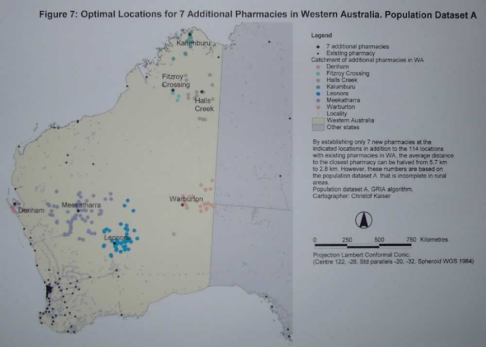
The Aboriginal Community Warburton has a notable population of 457 and neighbouring locations are also populated. But it is 848 km to the nearest pharmacy, which is in Kalgoorlie. This isolated situation contributes significantly to the overall travel distance. Therefore, every optimal configuration that adds between one to 20 pharmacies in WA contains Warburton as a new service location. Hence, the establishment of a service in Warburton does not depend on the total number of new facilities to be established. This is due to the used WA data; in general the localities in optimal configurations with different numbers of facilities are independent.

4.1.2 Population Dataset B
Population dataset B is more complete than A and also tries to include the disperse population in the rural areas. Hence population dataset B was used for most of the location/allocation calculations to gain more realistic results.

4.1.2.1 Establishing Additional Facilities
The existing pharmacies have an average distance of 9.9 km to the population of dataset B. By establishing five new facilities in Fitzroy Crossing, Halls Creek, Leonora, Meekatharra, and Warburton as shown on figure 8, this distance would be reduced by 1/3 to 6.6 km. Considering that already 114 locations in WA have pharmacies, the influence of these five proposed facilities is enormous. Establishing more new pharmacies increases the accessibility further, however the benefits per extra facility established decreases as shown in figure 9.

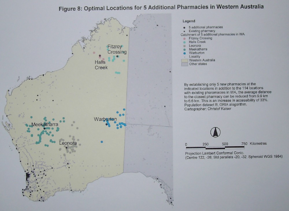
Figure 9: Effects of additional pharmacies. (GRIA with population dataset B)

To half the distance from 9.9 km to 4.9 km and doubling the accessibility, 17 new pharmacies need to be established in the locations shown on figure 10. Although both optimal configurations are independent, the configuration of 17 new facilities contains all locations suggested for the case of only five new ones.

4.1.2.2 Optimal Locations for the Existing Number of Pharmacies in WA
The pharmacies dataset contains 114 locations with at least one pharmacy in WA. Some locations have more than one pharmacy. However, the population dataset and the pharmacy dataset have different levels of aggregation. The population of an ‘Urban Centre or Locality’ (UCL) is always assigned completely to the central point of the UCL. But there can be more than one location with pharmacies in the UCL. So some locations have no known population but they have pharmacies. This leads to misinterpreted results if the given accessibility is compared with the optimal accessibility that could be achieved by distributing the given number of 114 pharmacy locations in a more optimal way. In the existing configuration, many pharmacies appear to be useless because they are at points without any population. So the optimisation algorithm will position these pharmacies to where they produce more benefits.

All pharmacies in WA are in a UCL or they are so close to one that they can be considered to be part of the UCL. This applies to six locations. Because the population of every UCL is assigned to exactly one locality, only pharmacy locations with a known population were counted. Doing this, the effective number of locations with one or more pharmacies comes down to 68.

The existing pharmacies and those in neighbour states lead to an average distance of 9.9 km for the population dataset B. But the same level of spatial accessibility could also be achieved with only 35 pharmacies in optimal locations as shown in figure 11.

For the given number of effectively 68 pharmacies as described above, Simulated Annealing found a better configuration as shown in figure 12 with an average distance of 5.7 km which is a increase in accessibility of 42%.

Further on, GRIA was run to position between 0 and 70 pharmacies in WA from scratch. The results for one to 70 pharmacies are graphed as average distance in figure 13. The average distance for the case of no pharmacy in WA is not infinite but as high as 1798 km because the demand is satisfied by pharmacies in South Australia and the Northern Territory. Again, the greatest increase in accessibility per facility established can be seen between configurations with small numbers of pharmacies. If the configuration already has a larger number of facilities, the change to a configuration with even more pharmacies has only a marginal positive impact on the accessibility.

Figure 13: Average distances for optimal configurations of 1-70 pharmacies in WA. Calculated using GRIA and population dataset B.

4.2 Comparison of the Algorithms
Two criteria to find good algorithms are the quality of the solution found and the time needed to calculate it.

4.2.1 Quality of the Solution
All six algorithms implemented, Add, Drop, GRIA, Teitz-Bart, the Genetic Algorithm and Simulated Annealing, were run to position 35 pharmacies in WA from the scratch, i.e. without any pre-existing facilities in WA. The average distances the different algorithms returned as results are graphed in figure 14.

Figure 14: Locating 35 pharmacies in WA. Results of different algorithms.

For this case, the Teitz-Bart algorithm and the Simulated Annealing approach based on Teitz-Bart found a slightly better solution than GRIA. The genetic algorithm could not offer a competitive solution, but it may come up with a better value if it is run over more iterations. The Drop approach was surprisingly good, but the Add heuristic was not successful.

Again all algorithms were tested for selecting 68 locations with the results shown in figure 15.

Figure 15: Results of different algorithms for locating 68 facilities.

In this run, Simulated Annealing produced the best result. It is better than the one for GRIA or Teitz-Bart. Although the difference between the results of GRIA and simulated annealing is very small, it shows that GRIA gets trapped in a local minimum for the WA data. However, due to its randomised character, it is not sure that SA will always be superior even if the same data is used.

The different algorithms were used to find optimal configurations for additional pharmacies in WA. The resulting costs are shown in figure 16. All of the algorithms, except the GA, came up with exactly the same quality of solutions. The GA produced slightly more expensive configurations in some cases.

Figure 16: Finding positions to establish additional facilities by using different algorithms. (Population data B)

4.2.2 Computation Time
The computation times of the developed pmedian program for the different algorithms implemented were measured with the WA data. The problem used was to locate 50 facilities from scratch but with fixed facilities in the neighbour states. The runtime of Add, Drop, GRIA, and Teitz-Bart depend on the data; the runtime of the Genetic Algorithm and the Simulated Annealing is also influenced by random factors within the algorithm as well as by a strong effect of the chosen parameters. So the times stated in table 1 are only to give an idea of the time needed by different algorithms. The average distance is included again to show the quality of the configuration found. The best solution is the one with the smallest distance.
 

 

Algorithm	Runtime (minutes)	Avg Distance (km)
Add/Greedy/Myopic	26	7.72
Drop	74	7.43
Teitz-Bart	53	7.43
GRIA	32	7.43
Genetic algorithm	126	9.65
Simulated Annealing	249	7.43

Table 1: Runtimes for locating 50 facilities from scratch in WA

5 Discussion

5.1 Effects of Service Locations on Accessibility in WA
Assuming the population dataset B is a good estimation of the distribution of the population in Western Australia, the results found show that the locations of facilities have a great impact on their accessibility. The distribution of pharmacies in WA is far from being optimal from a location theory point of view. Hence, the accessibility could be improved very significantly by either changing the position of existing pharmacies or establishing a small number of additional pharmacies. Already only five additional pharmacies in the right locations can reduce the average distance by 33%. However, relocating all the existing pharmacies to optimal positions would increase the accessibility much more. But relocating can be expected to raise resistance from different parties so that the patchy approach of establishing a few new pharmacies will be the more practicable way to go.

5.2 Suitability of the Different Algorithms
A variety of algorithms for the NP-hard p-median problem were implemented and used in this study. The Global/Regional Interchange Algorithm turned out to be the best both in terms of quality of the solution and computation time. Teitz-Bart does reasonably well but needs more time to return a solution. The genetic algorithm implemented for this study delivers useful results. However, in no case using the WA data it’s solution was superior to the one of GRIA. And the time needed was much longer. Simulated Annealing, implemented based on the Teitz-Bart algorithm, could once produce a slightly better result than GRIA or Teiz-Bart with the given WA data. Surprisingly, if only a small number of additional pharmacies are to be added to the existing ones, the naïve approaches of the add and drop algorithms could deliver a solution with the same quality as GRIA. It is supposed that this is because of the small number of pharmacies these are often not close together. This makes it unlikely that the regions assigned to different facilities influence each other. Hence, the location problem can be solved simply by putting facilities wherever the demand is greatest rather than considering that the sizes of the different catchments are determined by the spatial relationship of the new facilities.

5.3 Reasons for the Suboptimal Facility Positions
Based on the described data and the assumption that it is adequate to model the question of pharmacy locations as a p-median problem, it was found that the distribution of the facilities is clearly suboptimal in terms of accessibility.

This can be interpreted in two ways. Firstly, there might be more constraints in the real-world than in the plain p-median model. For example, the relationship between travel distance and cost or value of the objective function may not be linear. Road conditions may have an influence.

But secondly, when the p-median model is accepted as adequate, it can in fact be the case that the optimal configuration is not found in the real world. Shelley and Goodchild (1983) note that majority voting of the population does not lead to optimal configurations. So this widely accepted procedure of democratic decision-making can fail to find good positions for, as example, salutary public facilities. This is because voters tend to optimise or maximise their own benefits without seeing the overall effects.

If the pharmacies were established successively one by one and the places selected by the highest market demand, the configuration would be the one suggested by the add algorithm which is often sub-optimal. However, for the given data the add strategy still produces better results than the existing configuration.

It also must be considered that the population and hence the demand changes over time. The adjustment of the existing facilities to changing conditions might experience a delay.

The classical economist Adam Smith in 1776 (cited in Buchholz 1999, p. 21) was convinced that everyone ‘neither intends to promote the publick (sic) interest, nor knows how much he is promoting it … he intends only his own gain, and he is in this, as in many other cases, led by an invisible hand to promote an end which was not part of his intention.’ This, Smith believed, inevitably leads to the best overall solution for the whole economy. Obviously Smith did not know about the p-median problem. For this very problem, the uncoordinated establishing of facilities usually does not lead to the best overall solution.

6 Conclusion
Location theory is a well-established academic discipline. The algorithms available are likely to find the optimal or a very good solution for real world p-median problems. Other optimisation techniques such as genetic algorithms also produce reasonable results but are unlikely to outperform highly specialised p-median algorithms such as GRIA significantly. This is because genetic algorithms are a more generic concept that offers solutions for different problems rather than an algorithm that is only developed to solve the p-median problem. A comparison of the classical heuristic algorithms shows that GRIA is the best choice in terms of computation time and quality of the results. However, it was experienced once that the Simulated Annealing algorithm developed in this study found a slightly better solution than GRIA and Teitz-Bart.

The application of the pmedian program developed in this study on data of Western Australia shows a huge potential for optimising the spatial accessibility of pharmacies. Only establishing five pharmacies at the right locations can increase the spatial accessibility by 33%. This is because some of the remote areas of Australia are highly disadvantaged and could benefit enormously by only putting out a small number of new facilities due to savings of large travel distances. This study only utilised the locations of pharmacies in WA but other states and other services are believed to show similar results. However, it must be stressed that any location/allocation process is highly dependent on the quality and accuracy of the input data.

7 References
Ahuja, R.K., Magnati, T.L., and Orbin, J.B. 1993, Network flows : theory, algorithms, and applications Network flows : theory, algorithms, and applications, Prentice Hall, Englewood Cliffs, New Jersey, USA.

AUSLIG 2000, Feature Definitions [Internet], Available from <http://www.auslig.gov.au/products/digidat/v1_250k/usr_gide/ug00064.htm> [Accessed 10 July 2000].

Australian Bureau of Statistics 1997, CData96 [CD-ROM], Release 2 Final.

Beasley, J. E. 1985, A note on solving large p-median problems, European Journal of Operational Research, Vol. 21, pp. 270-273.

Chardaire, P., and Lutton, J. L. 1993, Using Simulated annealing to solve concentrator location problems in telecommunication networks, Applied Simulated Annealing, Springer, Berlin, pp. 175 – 199.

Christaller, W. 1933, Die Zentralen Orte in Süddeutschland, Jena, Translated by C. W. Baskin 1966, Central Places in Southern Germany, Prentice-Hall, Englewood Cliffs, New Jersey, USA.

Church, R. L. 1990, The Regional Constrained p-Median Problem, Geographical Analysis, Vol. 22(1), pp. 22 – 32.

Church, R. L., and Sorensen, P. 1996, Integrating normative location models into GIS: problems and prospects with the p-median model, Spatial Analysis: Modelling in a GIS Environment, GeoInformation International, Cambridge, pp. 167 – 183.

Commonwealth Department of Health and Aged Care 1999, Measuring Remoteness: Accessibility/Remoteness Index of Australia (ARIA), Occasional Papers: New Series No. 6.

Current, J. R., and Schilling, D. A. 1987, Elimination of Source A and B Errors in p-Median Location Problems, Geographical Analysis, Vol. 19(2), pp. 95 – 110.

Daskin, M. S., and Owen, S. H. 1999, Two New Location Covering Problems: The Partial P-Center Problem and the Partial Set Covering Problem, Geographical Analysis, Vol. 31(3), pp. 217 – 235.

Densham, P. J., and Rushton, G. 1992a, A More Efficient Heursitic for Solving Large P-Median Problems, Pares in Regional Science, Vol. 71(3), pp. 307 – 329.

Densham, P. J., and Rushton, G. 1992b, Strategies for solving large location-allocation problems by heuristic methods, Environment and Planning A, Vol. 24, pp. 280 – 304.

Densham, P. J., and Rushton, G. 1996, Providing spatial decision support for rural public service facilities that require a minimum workload, Environment and Planning B: Planning and Design, Vol. 23, pp. 553 – 574.

Feldman, E., Lehrer, F.A., and Ray, T.L. 1966, Warehouse location under continues economies of scale, Management Science, Vol. 12(9), pp. 670 – 685.

Fotheringham, A. S., Densham, P. J., and Curtis, A. 1995, The Zone Definition Problem in Location-Allocation Modeling, Geographical Analysis, Vol. 27(1), pp. 60 – 77.

French, R. 1994, Simulated Annealing [Internet], Available from < http://suif.stanford.edu/~rfrench/papers/bsthesis/section2_7_1.html >, Accessed 6 July 2000.

Goldberg, D. E. 1989, Genetic algorithms in search, optimisation, and machine learning, Addison-Wesley, Reading, Massachusetts.

Hakimi, S. L. 1964, Optimum Distribution of Switching Centers in a Communication Network and Some Related Graph Theoretic Problems, Operations Research, Vol. 13, pp. 462 – 475.

Kariv, O., and Hakimi, L. 1979, An Algorithmic Approach to Network Location Problems. II: The p-Medians, SIAM journal on applied mathematics, Vol. 37 (3), pp. 539 – 560.

Klincewicz, J. G. 1990, Solving a Freight Transport Problem using Facility Location Techniques, Operations Research, Vol. 38(1), pp. 99 – 109.

Kuehn, A., and Hamburger, M. J. 1963, A heuristic Program for Locating Warehouses, Management Science, Vol. 9, pp. 643 – 666.

Maranzana, F. E. 1964, On the Location of Supply Points to Minimize Transport Costs, Operation Research Quarterly, Vol. 15(3), pp. 261 – 270.

Metropolis, N., Rosenbluth, A. W., Rosenbluth, M. N., and Teller, A. H. 1953, Equation of State Calculations by Fast Computing Machines, The Journal of Chemical Physics, Vol. 21(6), pp. 1087 – 1092.

Murray, A. T., and Gottsegen, J. M. 1997, The Influence of Data Aggregation on the Stability of p-Median Location Model Solutions, Geographical Analysis, Vol. 29(3), pp. 200 – 213.

Narula, S. C., Ogbu, U. I., and Samuelsson, H. M. 1977, An Algorithm for the p-Median Problem, Operations Research, Vol. 25, pp. 709 – 713.

Nascimento, E. M., and Beasley, J. E. 1993 Locating Benefit Posts in Brazil, Journal of the Operational Research Society, Vol. 44(11), pp. 1063 – 1066.

Pelletier, J. 1998, More on Time Complexity of Algorithms [Internet], Available from <http://www.cs.ualberta.ca/~jeffp/c114/8morecmplxty/sld011.htm>, Accessed 18 July 2000.

Plesnik, J. 1987, A heuristic for the p-center problem in graphs, Discrete Applied Mathematics, Vol. 17, pp. 263 – 268.

Shelley, F. M., and Goodchild, M. F. 1983, Majority Voting and the Location of Salutary Public Facilities, Geographical Analysis, Vol. 15(3), pp. 205 – 211.

Smith, A 1776, Wealth of Nations. Cited in: Buchholz, T. G. 1999, New Ideas from Dead Economists, revised edition, Penguin Books, London.

Teitz, M. B., and Bart, P. 1968, Heuristic Methods for Estimating the Generalized Vertex Median of a Weighted Graph, Operations Research, Vol. 16, pp. 955 – 961.

Thünen, J. H. von 1826, Der Isolierte Staat in Beziehung auf Landwirtschaft und Nationalökonomie, Hamburg. Translation by Wartenberg, C.M. 1966, Isolated state, Oxford, Pergamon Press.

8 Appendix A: Manual for pmedian

Purpose
pmedian is a java program (JDK 1.1) to solve p-median problems. The source code is in a file called pmedian.java, the java executables are pmedian.class and pmedian$chromosome.class.

Input Data
All in/output is done using CSV text files. If the first line is non-numeric, it is ignored. So CSV headers do not have to be removed.

Distance Matrix
Every line of the distance matrix file should be in the following format:
LocID_from,LocID_to,distance

Eg:

3,5,24
4,3,42
4,4,0
…

All values must be integer. This format can be generated out of a binary matrix file using readod ( eg readod bin_file > mat.csv ). The matrix file is often very large in size. So it is good to copy it to a local drive (/tmp).

Demand or Population Data
Format:
LocID, demand
Eg

3,50
4,23
..

Candidates
All LocIDs that are suited to establish a facility. Format:
LocID

Eg

4
6
7
..

Command Line for pmedian
The programm is started the following command line:

java pmedian –ALGORITHM matrix_file demand_file candidates_file [#facilities_to_establish] [flags and parameters]

Algorithms
There is a choice of these implemented algorithms:
 

Algorithm Flag	Comments
-add (the same as –greedy or –myopic)	Greedy algorithm
-drop	Drop algorithm
-gria	GRIA algorithm. This is often the best choice.
-tb	Teitz-Bart algorithm.
-ga	A genetic algorithm. More parameters can be specified with the  –algoparam flag
-sa	Simmulated annealing. More parameters can be specified with the  –algoparam falg
-enum	Enumerative algorithm that guarantees to find the optimal solution. However, the runtime exceeds any limits for larger problems.
-cost	Calculates the cost only. The candidate file is used as a configuration.  –allocation and other flags still work. Do not specify the number of facilities to put when using the –cost option.

Flags
 

Flag	Comment
-nonverbose	Switches out additional output. pmedian should be run in the verbose mode from time to time or if using new data to see if it is ok and which demands are ignored because of problems with the matrix file. The output can be redirected with > filename at the end of the command line.
-output filename or -solution filename	Writes the result configuration to a file. These are the LocIDs of the best configuration found.
-allocation filename	Writes the allocation and distance of every demand point to a file. The format is: LocID_demand, LocID_allocated_to, distance So 3,5,56 means that LocID 3 is allocated to a facility at LocID 5 in a distance of 56. This flag also works for the -cost option. A unreasonable big distance (2147483648) indicates that the demand LocID was not allocated at all because the distance matrix does not offer a way from the demand point to a facility of the configuration. This usually happens if the road network is broken or some points are not connected to the network.
-allocall	Normally demand points with a demand of 0 are ignored because they do not influence the optimisation. With this flag set, they are processed anyway. This is useful if the allocation is written using –allocation and a map should be produced. So no points are un-allocated. However, it slows down the process. For large problems, it is best first to find the best configuration and than output the allocation in a separate run using the –cost option. So the optimisation is not slowed down by point with nil demand.
-fixed filename	The file specified is read and must hold a list of LocIDs in the format as the candidate file. These ‘fixed’ LocIDs are treated as facilities that exist but cannot be moved i.e. optimised. The use of this flag is for facilities in neighbour areas that also can satisfy demand or as a backdrop configuration if new additional facilities should be established.
-algoparam [parameters]	Specifies specific parameters for the –sa or –ga algorithms. For SA -algoparam starting_temp cooling_rate eg -algoparam 500000 0.999 For GA -algoparam population_size max_idle_iterations promote_best promote_crossover promote_mutation mutation_rate crossover_method eg -algoparam 200 500 0.02 0.68 0.3 0.1 4 promote_best, promote_crossover and promote_mutation must sum up to 1. Mutation_rate is the fraction of information that is changed randomly if a chromosome is mutated. crossover_method 4 appears to be the best.

Example Command Lines

java pmedian –gria matrix.csv population.csv candidates.csv 20 –fixed facilities_nt_sa –nonverbose –output gria_conf.txt >out_gria

to use GRIA to put out 20 facilities and write the resulting configuration to gria_conf.txt .

java pmedian –cost matrix.csv population.csv gria_conf.txt –fixed facilities_nt_sa –nonverbose –allocation gria_alloc.txt –allocall

to get the allocation of the configuration found by the first command.

Expected Runtime
Typical times needed by pmedian to solve a problem range between 10 an 200 minutes. Some hints about the progress can be gained if the verbose mode is used (i.e. –nonverbose is not set) and the redirected output is observed from time to time.

Helpful Unix commands
The flowing Unix commands are helpful to handle CSV files:
 

cut	to select one ore more columns
grep	to find lines containing a certain text
egrep	same as grep with regular expressions
sed	to perform text substitutions such as sed "s/ *//g" to remove spaces from the output file of readod. sed "s/$/,1" <in_csv >out_csv appends ,1 to each line. This can be used before importing a configuration (i.e. a list of LocIDs) into ArcView. However, a first line like "LocID","in_solution" must be added as well because ArcView expects a CSV header.
> outfile	In most cases the output of pmedian should be redirected to a file for further use. The total cost of the configuration found is written to the standard output. If the  –nonverbose option is used, this is the only line of the output.
tail filename head filename	Prints the end or beginning of a file.

Note: The Java program can be provided uppon request. See my homepage for my email address.